Openbox

Repeat calculations using arrays

You often want to repeat a set of calculations in your model. Here are some examples:

  • You might have several different products and need to calculate revenue by product and total revenue;
  • You have several scenarios, and you want to take the minimum and maximum value of some metric (e.g. IRR) over all scenarios;
  • You have three main types of asset: buildings, office equipment and other. Each type of asset has a different lifetime, and the purchase/ disposal profile will be different. You need to track capex, depreciation and disposals for each asset type, but report the total on your balance sheet.

Openbox allows you to do this easily.

It’s a two step process. First, write the calculations as if there was only one product/ scenario/ asset class. Then tell Openbox that some of the inputs need to be repeated for all items in an ‘array’ that you define. An array is just a list e.g. “buildings, equipment,other” or “upside, base case, downside”. Openbox will repeat the inputs, and any calculations that depend on those inputs, directly or indirectly. So if you tell Openbox that the input “asset life” varies by type of asset, essentially all the fixed assets section will be repeated three times.

You might be wondering at this point how we stop the model becoming very large. Later in this article we’ll see how to consolidate calculations so that not everything in the model is repeated. But first, let’s look at how to create an array.

How to create an array

To create an array, click “Manage Arrays” in the Ribbon. You can then add a new array, or edit or delete an existing one.
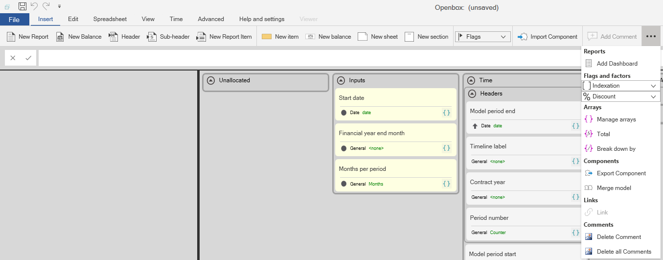
To apply an array to an input, select the input on the diagram and then click the ‘{ }’ icon on it. This will ask you if you want to add a new array to the item, or to manage the existing arrays.

If you click “New”, you’ll see a window like the one below.
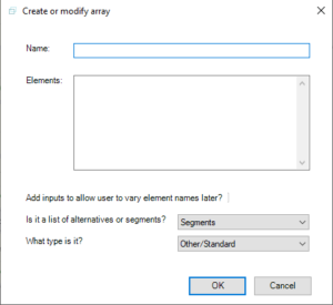
To create a new array, you need to tell Openbox a few things about it:

  • Its name. This can be any text
  • The elements. This can be a list of text items (e.g. ‘high case’, ‘central case’,’ downside case’) or a series of numbers (e.g. 1:10 represents all the numbers from 1 to 10 inclusive) or dates.
  • Whether the elements are numbers, dates or just text (“standard”).
  • Whether the elements of the array are ‘alternatives’ or ‘segments’. This affects how they will be shown on reports.

Let’s explain a little more about alternatives and segments. “‘Alternatives” means that the elements are different possible values for the input, but that it does not make sense to add them together. “Segments” means that it does make sense to add them together. For example, a list of scenarios would be alternatives, whereas a list of products would be segments. This is because you could sensibly add together say the revenue for each product to get total revenue but adding together the revenue for each scenario wouldn’t make sense. 

Openbox will put all segments on the same report, but will create a separate report for each alternative. So if you have three scenarios (“alternatives”) for say revenue, which appears on the income statement, you get three income statements. But if you have revenue for three business units, which are alternatives, you get the revenue for all three units on the same income statement.

Once you click ‘OK’, Openbox will add the array to the dropdown list. The selected input, and any calculations that depend on it, will now have multiple values, one for each item in the array.

You can add the array to other inputs by selecting the input, clicking the ‘{ }’ and then ticking or unticking the arrays you want to apply.

And once you have added arrays to inputs, that is it. Remember that Openbox automatically works out which other calculations need to vary. For example, if “Asset lifetime” varies by the “Asset class” array, then “Depreciation”, “Net book value” and so on will need to vary too.

This can become complex. Openbox will check and warn, during validation, if it finds any array inconsistencies. In particular, if a balance varies by some array, all the flows into it need to vary by that array too. To give an example, suppose you had three business units and wanted “Cash” to be tracked separately for each one – to vary by business unit. And suppose it is calculated as opening cash plus net cashflow. Then net cash flow would have to be specific to the business unit too – it would have to vary by business unit.

Multiple arrays

You can also combine several arrays in one variable. For example, you might want to split “Revenue” by product, but also by geography, so you can look at US sales of product 1, European sales of product 2 and so on.

To do this, create a “Product” array, say “Product1,Product2,Product3″, and a “Geography” array, say “US,Europe,Asia”. Click on the desired input, “Sales forecast” say, and then ‘{ }’. Make sure both “Product” and “Geography” are ticked.

Now the “Revenue” item will have 3 x 3 = 9 values, one for each possible combination of product and geography. Any items that depend on it will automatically have nine values as well, unless you deliberately ‘consolidate’ an array (see below).

Note that using multiple arrays can quickly lead to a very large number of calculations – use caution!

Consolidating values across an array

Often when you have scenarios or arrays, you want to combine or compare the values in some way. You might want to sum revenue by product line to get total revenue, or to look at the minimum NPV achieved across all scenarios.

To do this, use the special functions SUMOVER, MAXOVER, MINOVER and MEANOVER. The first argument is the array you want to take the sum, max, min or average over. The second argument is the variable you are summing/ maxing/ mining. For example “SUMOVER([revenue by product], “product”)” is the total revenue across all product lines.

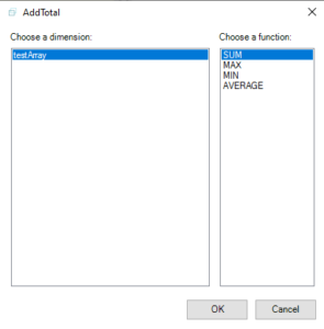
The easiest way to do this is to select the item you want to consolidate, and then click “Insert”, three dots for the advanced menu, then the “Total” button . This will ask you how you want to consolidate, and then will add a new calculation block that does the consolidation.
You can also go the other way by clicking the “Break down by” button, which is beside the Totals button. This takes an existing calculation and allows you to make it vary by array. Here’s how it works:

  1. Select the calculation. For example, select “Fixed assets
  2. Click “Break down by
  3. Select the array you want to break down by.
  4. You’ll be asked how you want to consolidate the array – usually, by SUMming.
  5. Openbox will then work out what the inputs are that affect “Fixed assets”. At least one of them must vary by the array you specified in step 3, if Fixed Assets is to vary by that array. Tick the input(s) that vary by this array and click OK.
  6. Openbox modifies the inputs as specified. It also adds a new calculation that works out Fixed Assets for each member of the array you chose, and sets “Fixed Assets” to be the consolidation of those items.

Set Number Formats

When Openbox creates your Excel model, it applies a number format to every input, calculation and output. That format is based on units. So for example, anything with units of “%” gets a % format, anything with units of “$” gets a currency format and so on. The default is the “General” number format.

You can customise the number formats at different levels.

Individual calculations

First of all, you can set the number format for an individual calculation or input.


If you don’t see this, try pressing Ctrl+Shift+H or clicking the “Show icons” button in the Ribbon.

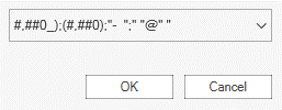
The “Depreciation” item above has a number format of “General”. Click on that, and you will see a popup box as below:

Either pick a format from the dropdown list, or type a new custom format and press Enter/ Return. Openbox uses the same number formats as Excel Available number formats in Excel (microsoft.com)

All calculations of a certain type

You can also tell Openbox to apply a number format to all calculations of a certain type – that is, with a particular unit. For instance, suppose anything with units of $ should be formatted as 0.00 so you can see dollars and cents.

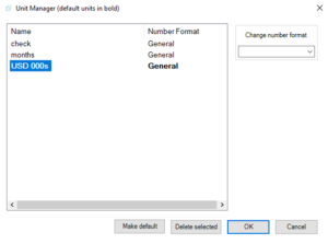
To do this, use the “Manage units” button. This will show you a list of every unit in the model.

Click on the one you want to change. Then go to the “Change number format” section. You can either select one of the standard formats from the dropdown list, or type a custom format in the box.

If there is a number format set for an individual calculation, this overrides any number format associated with units.

Troubleshooting

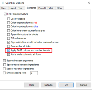
If number formats are not working as you expect, it may be because of the “Apply FAST number formats” option. This applies certain standard formats, like 0.0000 for discount rates and indexes. You can turn this off in the Options window:

Create and customise a report


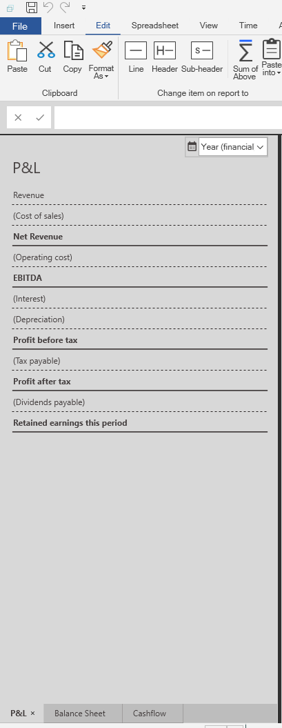
Reports are shown on the left hand side of the screen, like this:

Note that you can hide and show the reports section. Click “View” then the three dots at the end, then you can toggle the reports section by clicking the “Report” button under “Show/hide“. So if the reports section is not visible, try clicking this button once.

You can add a new, blank, report, or create one based on a list of names from an Excel file.

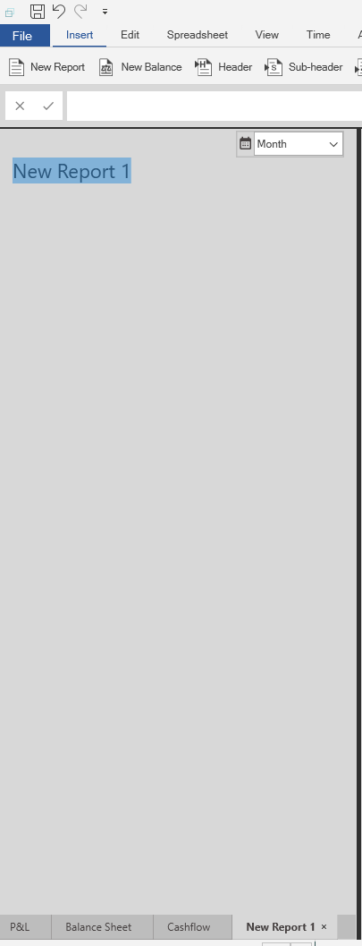
To create a new, blank, report click “New Report” on the “Insert” menu. A new report will appear like this:

The default name, “New Report 1” is highlighted so you can quickly type a new name for it.

Note that there are tabs at the bottom, much like spreadsheet tabs. Each tab represents a single report sheet in the financial model that will be produced. You can delete tabs using the “x” icon on each one, and scroll in a similar way to in Excel.

You can also add a new report from a list in Excel. First copy the list in Excel. Then in Openbox, click “Edit“, three dots at the end,  “Paste Into” and “New report“. Note that you can also paste into an existing report by clicking the “current report” option.

Openbox will create report lines with the desired names. It will ask you if the items are balances or not – simply click ‘yes’ to create a balance sheet or ‘no’ otherwise. If you are unsure, click ‘no’. You can always change the items later using the buttons in “Edit” as highlighted below.

Openbox will also add placeholders for each new report line in the main, calculation, window.

Add headers to each sheet

Openbox can insert standard header rows on each sheet – for example, the start and/ or end of each period in the model, or the period number.

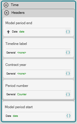
To insert headers, put the desired calculations in the ‘Headers’ section of the ‘Time’ sheet. They will then appear in the header on each sheet, in the same order as in the headers section.

For example, the model created from the diagram below will have ‘Model period end’ as the first row of the header, then the ‘Period number’ and so on.

The items in ‘Headers’ are standard calculations, so you can re-order them, remove them, or add new ones.

Note that you will have to update your Excel template file as well, to make sure there are enough rows in the sheet headers, and that they are formatted as you want. Openbox will warn you if for example, you try to put five headers into an Excel template with space only for four.

For example, here is the sheet header section in the standard “Gridlines template.xlsx” file that comes with Openbox. There is space for four headers, and formatting applied to “Timeline label”.

Set the model timeline(s)

Unlike an Excel model, where the time basis is built in through the column structure, formulas and headings, time is effectively an input to an Openbox model. So you can easily change it part way through model development.

An Openbox model can have several timelines: a primary timeline, a secondary one, and separate one(s) for each report. Here’s how that works.

All models have a primary or main time axis. This spans the whole period that the model covers. Each model can also – but doesn’t have to– have a secondary time axis. This secondary axis is more detailed than the first and applies to only part of the period covered by the model. 

Let’s take an example. You want a model for a new power plant. The model needs to start on 1 January 2025 and run to 31 December 2049. Most of the model will be on a quarterly basis. Construction, which is due to start in 2025 and take 12 months, needs to be modelled on a monthly basis, however. So, you tell Openbox that the primary time axis is quarterly, from 1 January 2025 to 31 December 2049, and that the secondary axis is monthly, from 1 January 2025 to 31 December 2021. All calculations for construction will be done on a monthly basis, and the results converted automatically (using standard Excel formulas) to a quarterly basis, so they can feed into the main quarterly part of the model.

This is separate to the time axis for any reports. Each report can be on any time axis (as long as it is no more detailed than the primary axis). This means that you can have yearly reporting (on calendar, model or financial year basis) in a model with a monthly construction period and quarterly operational period, and Openbox will handle all the month to quarter to annual conversions for you. Or you can have one report on an annual basis, one on a quarterly basis and so on.

You can also tell Openbox that you want to see multiple report timelines. Suppose you have a quarterly model, and your client wants to see reports on a semi-annual and annual basis. Create the report, set the time axis to “Yearly” and then tick the “Add reports for all timelines” box on the “Layout” options tab. When you create the preview spreadsheet again you will see quarterly, semi annual and annual versions of the same report.

Settings menu

You tell Openbox what the timelines are through ‘Time’, ‘Settings’ in the menu bar. 


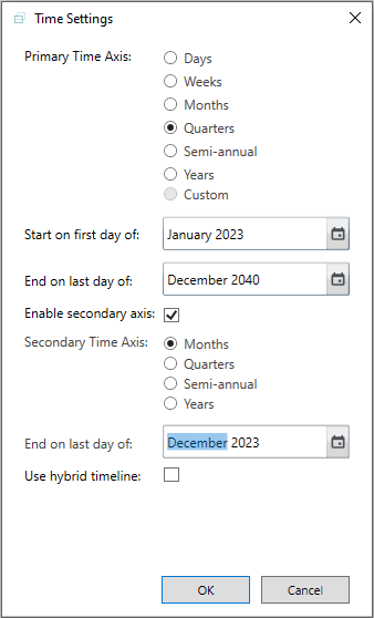
When you click on settings, you will see the main time settings window, as shown below.


Parts of the settings window

In the dialog box above, the top part sets the primary time axis. You must set this for any model. A time axis has a start date, an end date, and a periodicity (e.g. quarterly) within that. The only restriction here is that the end date must be a whole number of time periods after the start date. For example, you can’t have a quarterly model that starts in January and finishes in May.

If you want a secondary axis, tick the ‘Enable secondary axis’ box. You can then choose the start date, end date and periodicity of the secondary axis on the right-hand side.

There are some restrictions on the secondary axis. You can think of the secondary axis as like ‘zooming in’ on part of the period covered by the model, and the restrictions reflect that.

First, it must be more detailed than the primary. You can have a monthly secondary axis in a model with an annual primary axis, but not the other way round. 

Second, the dates for the secondary axis must also be within the dates for the primary axis. The start date is automatically the same as the start date for the primary axis, and the end date must be on or before the end date for the primary axis. You cannot ‘zoom in’ on a time period that is not actually part of the period covered by the model.

Note that the end date must be the end date of one of the periods of the primary axis. This avoids complex formulas for taking values from the secondary axis part of the model and transferring them to the primary part.

Finally, please note that the secondary timeline option is not available when the primary timeline is days or weeks. This is because of the complexity of converting from (say) weeks to years. We expect to offer this in a future update.

Hybrid timelines

You might have spotted that there’s a “Use hybrid timeline” box in the settings window. 

By default, Openbox creates separate worksheets for primary and secondary calculations and inputs. So if you have a quarterly primary axis and a monthly secondary axis, then some sheets will have quarterly dates across the top, and some will have monthly. But they won’t have both.

A “hybrid” timeline includes both timelines on the same sheet. So in our example, the dates would start as monthly, and change to quarterly after the secondary time axis finished.

This only affects how the model is laid out – it does not affect the results – and so is purely personal (or client) preference.

Timeline for reports

Good practice is that the model should calculate on the most granular or detailed basis required, and then this should be consolidated into reports, which might be on a less detailed basis. When setting the time in this dialog box, always choose the most granular time basis that the model will need. You can change the time basis of reports later – it is easy to have a model that calculates monthly, but which produces semi-annual or annual reports.

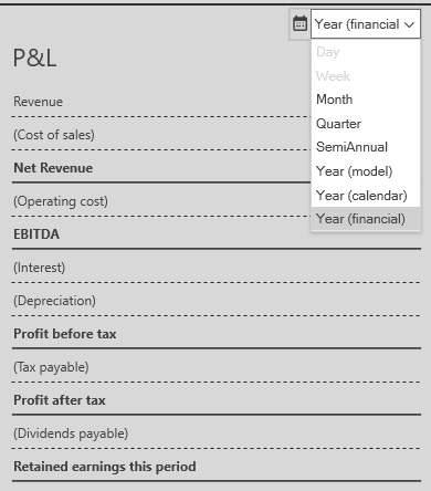
To change the timeline of a report, select the report in the reports window, on the left, and click the time dropdown at the top right of the report.

Note that day and week are greyed out, because reports cannot be on a more detailed timeline than the main model.

What are the keyboard shortcuts in Openbox?

Ctrl+…

0 In Focus mode, re-centre on the selected item
1 Change the selected line item to a balance
2 Change the selected line item to a flow
3 Change the selected line item to a flag
4 Change the selected line item to a Report line
5 Change the selected line item to a Report heading
6 Change the selected line item to a Report heading
A Select all (visible) items
B Add a new balance to the model
Copy
Find
New sheet/list
I Import a component
M Merge two items. If two items are selected, it will merge those two. Otherwise, it will ask which ones to merge.
Add a new item to the model
Open
Save
Paste
Undo
Collapse all sections
+ Expand all sections
% Apply the % style to the selected item(s)
[ If you select a cell with the name of a calculation in the preview window, Ctrl + [ will show that calculation in Focus mode in the main window

Ctrl+shift+…

Key  
1 Add a new heading to the current report
2 Add a new sub-heading to the current report
New balance item on report
C Toggle whether the selected item is constant or not
Add a new flag
G Create a new section from the selected items
H Show/ hide the icons that show additional information about each item, such as its units
I Move the selected item to the Inputs sheet, or all placeholders in a sheet or section if one is selected, or all placeholders if nothing is selected
L Apply Date units to the selected  item(s)
Swap mode
New report line
O Add a comment to the selected item(s)
P Toggle the Preview pane on or off
Split an item in two
T Add a new line item which calculates the total of the selected item, over some array
U Set the units for the selected item(s)
W Mark calculations in Excel as ‘to be deleted’. Openbox will remove them from the diagram the next time you go into Edit mode.
Z Mark calculations in Excel as ‘new or updated’. Openbox will read them and update the diagram to reflect them, the next time you go into Edit mode.
, (comma) Apply the standard number format to the item
. (dot) Apply the factor units, and command, to the selected item(s)

Other shortcuts

Key Action
F2  Edit formula of selected item
Ctrl+F2 Edit the name of the selected item
F9  Preview model
Shift +F9  Validate and preview model
Ctrl+Shift+F9 Validate the model and open it in Excel
Home  Go to home point on schematic
Arrow keys Change the selection to the item above/ below/ to the left or right
Ctrl+Arrow keys Move the selection up, down or left and right to other sheets/ sections
Alt+Down key In the preview, add a dropdown list of all items in the model to the current cell, and insert a link to the item you click on
[ Pressing [ while editing a formula brings up a list of all line items. You can then search by typing part of the name eg typing ‘cash’ brings up things like ‘cash balance’, ‘opening cash’, ‘cash available for debt service’.

Quick Start – building your first model

This is a walk through to show you how to build a simple project finance model using Openbox.

OpenBox is designed to be flexible, but for creating new models we find that a four stage process works well:

  1. Choose the TYPE of model
  2. IMPORT components to do the main calculations
  3. CUSTOMISE for things that are very project or client specific
  4. Send the model to EXCEL

Stage 1: Type of Model

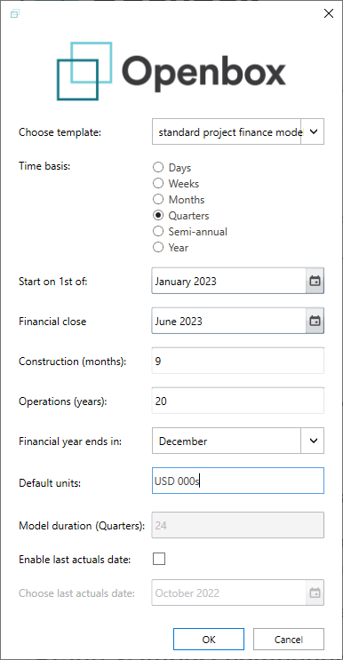
Open Excel and click “Openbox” then “New”. You will see a dialog like the one below.

Click on the “Template” dropdown and choose “standard project finance model.obz

Then type “USD 000s” in the “Default units” box, and set the start date to January 2023, financial close to June 2023, construction duration to 9 months and operations duration to 20 years. Click “Quarters” under “Time basis“. Then click OK.

The main Openbox screen will appear. You can then move on to the next stage –  importing components.

 Stage 2: Import components

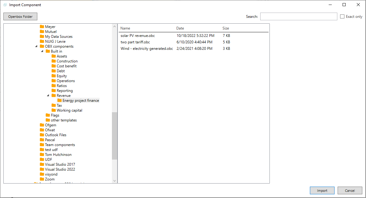
Let’s make this a solar PV model. To import a component, click “Ctrl+i“. You should see a screen like this.

Click the “Openbox folder” button at the top. Then select the “Built in” directory, then “Revenue” then “Energy project finance”. Select the “solar PV revenue.obc” file and click “Import”.

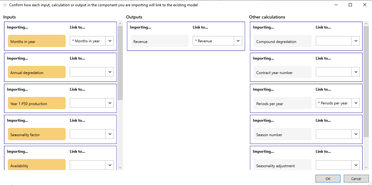
You will then see another screen like this:

This is asking how to link the component to the existing model. We’ll discuss it in more detail another time – just click “OK” for now.

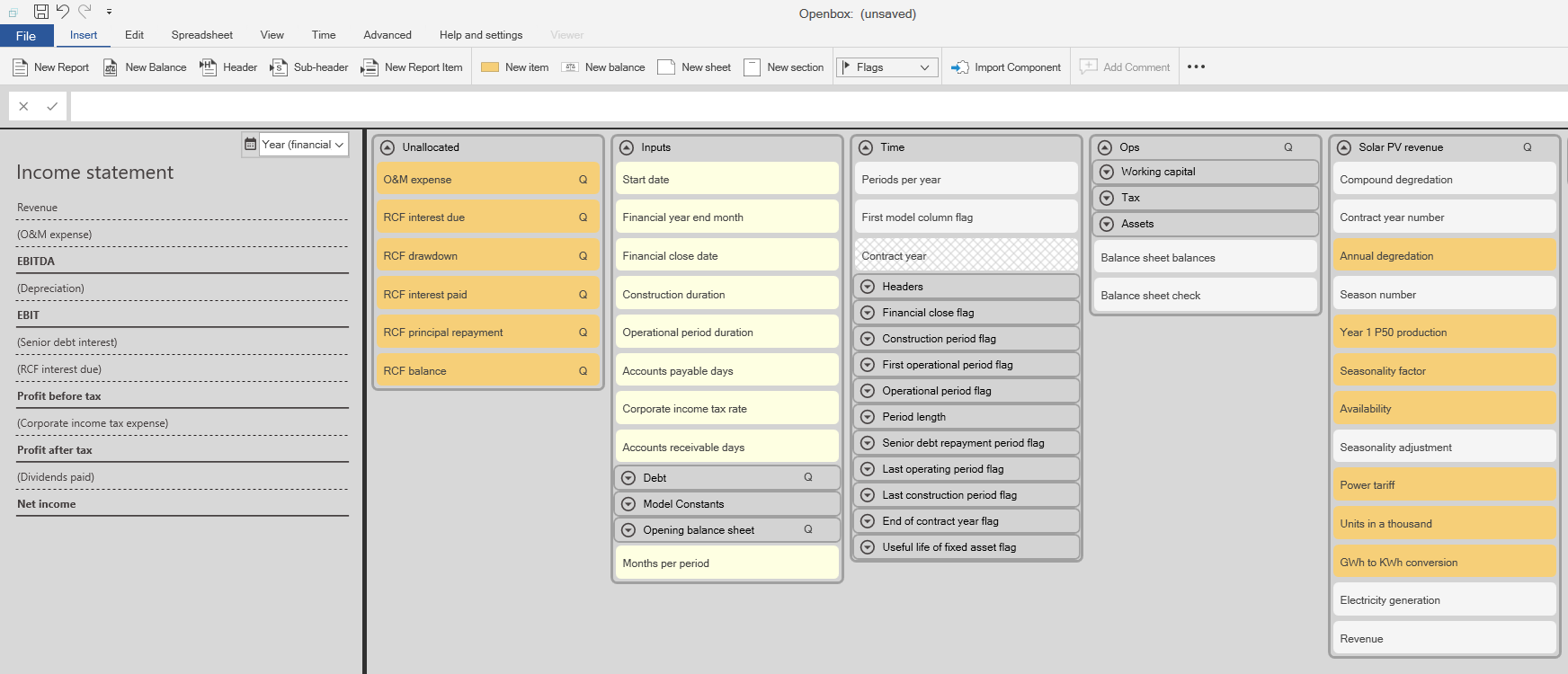
You’ll see that “Revenue” has disappeared from our “Unallocated” list, and there’s a new list on the right hand side. The “Revenue” calculation is now at the bottom of that list. The screen should look something like this:

Now click “Ctrl+i” again, then select the “Built in” folder, then “Operations” then “Project finance” and select the “simple fixed opex.obc” file. Click “Import” then “OK” at the next window.

Finally, the revolving credit facility. Click “Ctrl+i” again, then select the “Built in“, then the “Debt” folder, then the “RCF.obc” file. Click “Import” then “OK“.

That deals with almost the whole “Unallocated” (there’s one opening balance, which we can ignore for now), so now we can move on to customisation.

Stage 3 – Customisation

Let’s suppose we want to set the RCF interest rate. Go to the top of the RCF list on the screen and click “All in RCF annual interest rate”.

Typically, an interest rate will be a base rate plus a margin. Let’s do that here.

Press F2 to go to the formula bar, just like in Excel. Type “[RCF base rate] + [RCF interest margin]“. Press Enter.

Now RCF base rate and RCF interest margin are not in the diagram yet. Openbox will ask you if you want to add them. Note that you can say “Yes, always” and Openbox will do this automatically in future. For now, just click “Yes”.

Next it asks you if you want the base rate to be a constant. Let’s suppose not – maybe we expect it to increase in future. Click “No“.

And the same question for the margin. Let’s suppose that this is fixed. So click “Yes“.

Let’s tidy up by moving any remaining placeholders to the units sheet. Click “Edit” then the three dots “…” and then “Placeholders to inputs“.

And let’s tidy up the units by applying the default units to anything that doesn’t already have units.

Click  the three dots again, then “Apply default” and “To entire model“.

Now all that remains is to tell Openbox to translate the model to Excel.

Click “Spreadsheet” menu, then “Build Model“. 

We haven’t saved the model yet, and we need to do that before building. So Openbox asks us for a name to save it under. Type a name for the model e.g. “Quick start model v1” and press “Save“.

Openbox will pop up a few messages alerting you to various possible issues with the model. We can ignore them for this quick start, so just click “OK” to any messages that appear. For more information, see What checks does Openbox do as part of validation?

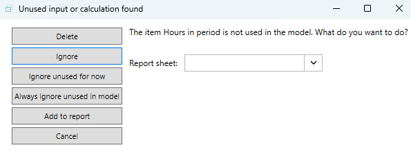
You’ll also see a message saying “Unused input or calculation found”. Again, for a real model, we’d want to check this out, but just click “Ignore unused for now“.

Once Openbox has done all its pre-build checks, it will ask you for a name for the Excel file. It will suggest a name but you can make it anything you like.

A progress bar will appear, showing the steps Openbox takes to create your Excel model, and then the model will appear in Excel.

Because Openbox needs to communicate with Excel during this process, we recommend that you don’t work in Excel while Openbox is building the model.

Once the model appears in Excel and the progress bar disappears, the Excel model is ready for use. You can use it just like any other Excel model.